Lesson 3

Corresponds to chapter 4 of the book.

Book notes

Tensor jargon - rank is the number of dimensions, shape is the size of each of the axes.

A PyTorch tensor is nearly the same thing as a NumPy array, but with an additional restriction that unlocks some additional capabilities. It's the same in that it, too, is a multidimensional table of data, with all items of the same type. However, the restriction is that a tensor cannot use just any old type—it has to use a single basic numeric type for all components. For example, a PyTorch tensor cannot be jagged. It is always a regularly shaped multidimensional rectangular structure.

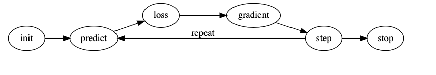
To be more specific, here are the steps that we are going to require, to turn create a machine learning classifier:

Initialize the weights.
For each image, use these weights to predict whether it appears to be a 3 or a 7.
Based on these predictions, calculate how good the model is (its loss).
Calculate the gradient, which measures for each weight, how changing that weight would change the loss
Step (that is, change) all the weights based on that calculation.
Go back to the step 2, and repeat the process.
Iterate until you decide to stop the training process (for instance, because the model is good enough or you don't want to wait any longer).

tensor.backward() calculates the gradient of the function at a particular value.

Example:

def f(x): return x**2

xt = tensor(3.0).requires_grad_() # requires_grad mentions that pytorch should calculate gradients
yt = f(xt)
yt.backward()
grad = xt.grad

Book notes